10 minutes to xorbits.pandas#
This is a short introduction to xorbits.pandas which is originated from pandas’ quickstart.
Customarily, we import and init as follows:
In [1]: import xorbits

In [2]: import xorbits.numpy as np

In [3]: import xorbits.pandas as pd

In [4]: xorbits.init()
Object creation#
Creating a Series by passing a list of values, letting it create a default integer index:
In [5]: s = pd.Series([1, 3, 5, np.nan, 6, 8])

In [6]: s
Out[6]:
0    1.0
1    3.0
2    5.0
3    NaN
4    6.0
5    8.0
dtype: float64
Creating a DataFrame by passing an array, with a datetime index and labeled columns:
In [7]: dates = pd.date_range('20130101', periods=6)

In [8]: dates
Out[8]:
DatetimeIndex(['2013-01-01', '2013-01-02', '2013-01-03', '2013-01-04',
               '2013-01-05', '2013-01-06'],
              dtype='datetime64[ns]', freq='D')

In [9]: df = pd.DataFrame(np.random.randn(6, 4), index=dates, columns=list('ABCD'))

In [10]: df
Out[10]:
                   A         B         C         D
2013-01-01  0.874899  0.120937 -1.095859  0.290422
2013-01-02  0.846309  0.635939  0.526437 -0.170163
2013-01-03 -1.557106 -0.469371 -0.987265 -0.697665
2013-01-04  0.418433  1.245349  0.831575 -1.131535
2013-01-05 -1.159543 -0.484924 -1.059262  1.297614
2013-01-06  2.690274  1.552518 -1.969173 -1.521865
Creating a DataFrame by passing a dict of objects that can be converted to series-like.
In [11]: df2 = pd.DataFrame({'A': 1.,
   ....:                     'B': pd.Timestamp('20130102'),
   ....:                     'C': pd.Series(1, index=list(range(4)), dtype='float32'),
   ....:                     'D': np.array([3] * 4, dtype='int32'),
   ....:                     'E': 'foo'})
   ....:

In [12]: df2
Out[12]:
     A          B    C  D    E
0  1.0 2013-01-02  1.0  3  foo
1  1.0 2013-01-02  1.0  3  foo
2  1.0 2013-01-02  1.0  3  foo
3  1.0 2013-01-02  1.0  3  foo
The columns of the resulting DataFrame have different dtypes.
In [13]: df2.dtypes
Out[13]:
A           float64
B    datetime64[ns]
C           float32
D             int32
E            object
dtype: object
Viewing data#
Here is how to view the top and bottom rows of the frame:
In [14]: df.head()
Out[14]:
                   A         B         C         D
2013-01-01  0.874899  0.120937 -1.095859  0.290422
2013-01-02  0.846309  0.635939  0.526437 -0.170163
2013-01-03 -1.557106 -0.469371 -0.987265 -0.697665
2013-01-04  0.418433  1.245349  0.831575 -1.131535
2013-01-05 -1.159543 -0.484924 -1.059262  1.297614

In [15]: df.tail(3)
Out[15]:
                   A         B         C         D
2013-01-04  0.418433  1.245349  0.831575 -1.131535
2013-01-05 -1.159543 -0.484924 -1.059262  1.297614
2013-01-06  2.690274  1.552518 -1.969173 -1.521865
Display the index, columns:
In [16]: df.index
Out[16]:
DatetimeIndex(['2013-01-01', '2013-01-02', '2013-01-03', '2013-01-04',
               '2013-01-05', '2013-01-06'],
              dtype='datetime64[ns]', freq='D')

In [17]: df.columns
Out[17]: Index(['A', 'B', 'C', 'D'], dtype='object')
DataFrame.to_numpy() gives a ndarray representation of the underlying data. Note that this
can be an expensive operation when your DataFrame has columns with different data types,
which comes down to a fundamental difference between DataFrame and ndarray: ndarrays have one
dtype for the entire ndarray, while DataFrames have one dtype per column. When you call
DataFrame.to_numpy(), xorbits.pandas will find the ndarray dtype that can hold all
of the dtypes in the DataFrame. This may end up being object, which requires casting every
value to a Python object.
For df, our DataFrame of all floating-point values,
DataFrame.to_numpy() is fast and doesn’t require copying data.
In [18]: df.to_numpy()
Out[18]:
array([[ 0.87489935,  0.12093696, -1.09585858,  0.29042226],
       [ 0.84630881,  0.63593913,  0.52643706, -0.17016255],
       [-1.5571064 , -0.46937097, -0.98726518, -0.69766526],
       [ 0.41843323,  1.24534929,  0.831575  , -1.13153481],
       [-1.15954295, -0.48492443, -1.05926199,  1.29761389],
       [ 2.69027364,  1.55251794, -1.96917266, -1.52186538]])
For df2, the DataFrame with multiple dtypes, DataFrame.to_numpy() is relatively
expensive.
In [19]: df2.to_numpy()
Out[19]:
array([[1.0, Timestamp('2013-01-02 00:00:00'), 1.0, 3, 'foo'],
       [1.0, Timestamp('2013-01-02 00:00:00'), 1.0, 3, 'foo'],
       [1.0, Timestamp('2013-01-02 00:00:00'), 1.0, 3, 'foo'],
       [1.0, Timestamp('2013-01-02 00:00:00'), 1.0, 3, 'foo']],
      dtype=object)
Note
DataFrame.to_numpy() does not include the index or column
labels in the output.
describe() shows a quick statistic summary of your data:
In [20]: df.describe()
Out[20]:
              A         B         C         D
count  6.000000  6.000000  6.000000  6.000000
mean   0.352211  0.433408 -0.625591 -0.322199
std    1.543966  0.861238  1.076638  1.025418
min   -1.557106 -0.484924 -1.969173 -1.521865
25%   -0.765049 -0.321794 -1.086709 -1.023067
50%    0.632371  0.378438 -1.023264 -0.433914
75%    0.867752  1.092997  0.148012  0.175276
max    2.690274  1.552518  0.831575  1.297614
Sorting by an axis:
In [21]: df.sort_index(axis=1, ascending=False)
Out[21]:
                   D         C         B         A
2013-01-01  0.290422 -1.095859  0.120937  0.874899
2013-01-02 -0.170163  0.526437  0.635939  0.846309
2013-01-03 -0.697665 -0.987265 -0.469371 -1.557106
2013-01-04 -1.131535  0.831575  1.245349  0.418433
2013-01-05  1.297614 -1.059262 -0.484924 -1.159543
2013-01-06 -1.521865 -1.969173  1.552518  2.690274
Sorting by values:
In [22]: df.sort_values(by='B')
Out[22]:
                   A         B         C         D
2013-01-05 -1.159543 -0.484924 -1.059262  1.297614
2013-01-03 -1.557106 -0.469371 -0.987265 -0.697665
2013-01-01  0.874899  0.120937 -1.095859  0.290422
2013-01-02  0.846309  0.635939  0.526437 -0.170163
2013-01-04  0.418433  1.245349  0.831575 -1.131535
2013-01-06  2.690274  1.552518 -1.969173 -1.521865
Selection#
Note
While standard Python expressions for selecting and setting are
intuitive and come in handy for interactive work, for production code, we
recommend the optimized xorbits.pandas data access methods, .at, .iat,
.loc and .iloc.
Getting#
Selecting a single column, which yields a Series, equivalent to df.A:
In [23]: df['A']
Out[23]:
2013-01-01    0.874899
2013-01-02    0.846309
2013-01-03   -1.557106
2013-01-04    0.418433
2013-01-05   -1.159543
2013-01-06    2.690274
Freq: D, Name: A, dtype: float64
Selecting via [], which slices the rows:
In [24]: df[0:3]
Out[24]:
                   A         B         C         D
2013-01-01  0.874899  0.120937 -1.095859  0.290422
2013-01-02  0.846309  0.635939  0.526437 -0.170163
2013-01-03 -1.557106 -0.469371 -0.987265 -0.697665

In [25]: df['20130102':'20130104']
Out[25]:
                   A         B         C         D
2013-01-02  0.846309  0.635939  0.526437 -0.170163
2013-01-03 -1.557106 -0.469371 -0.987265 -0.697665
2013-01-04  0.418433  1.245349  0.831575 -1.131535
Selection by label#
For getting a cross section using a label:
In [26]: df.loc['20130101']
Out[26]:
A    0.874899
B    0.120937
C   -1.095859
D    0.290422
Name: 2013-01-01 00:00:00, dtype: float64
Selecting on a multi-axis by label:
In [27]: df.loc[:, ['A', 'B']]
Out[27]:
                   A         B
2013-01-01  0.874899  0.120937
2013-01-02  0.846309  0.635939
2013-01-03 -1.557106 -0.469371
2013-01-04  0.418433  1.245349
2013-01-05 -1.159543 -0.484924
2013-01-06  2.690274  1.552518
Showing label slicing, both endpoints are included:
In [28]: df.loc['20130102':'20130104', ['A', 'B']]
Out[28]:
                   A         B
2013-01-02  0.846309  0.635939
2013-01-03 -1.557106 -0.469371
2013-01-04  0.418433  1.245349
Reduction in the dimensions of the returned object:
In [29]: df.loc['20130102', ['A', 'B']]
Out[29]:
A    0.846309
B    0.635939
Name: 2013-01-02 00:00:00, dtype: float64
For getting a scalar value:
In [30]: df.loc['20130101', 'A']
Out[30]: 0.8748993500910293
For getting fast access to a scalar (equivalent to the prior method):
In [31]: df.at['20130101', 'A']
Out[31]: 0.8748993500910293
Selection by position#
Select via the position of the passed integers:
In [32]: df.iloc[3]
Out[32]:
A    0.418433
B    1.245349
C    0.831575
D   -1.131535
Name: 2013-01-04 00:00:00, dtype: float64
By integer slices, acting similar to python:
In [33]: df.iloc[3:5, 0:2]
Out[33]:
                   A         B
2013-01-04  0.418433  1.245349
2013-01-05 -1.159543 -0.484924
By lists of integer position locations, similar to the python style:
In [34]: df.iloc[[1, 2, 4], [0, 2]]
Out[34]:
                   A         C
2013-01-02  0.846309  0.526437
2013-01-03 -1.557106 -0.987265
2013-01-05 -1.159543 -1.059262
For slicing rows explicitly:
In [35]: df.iloc[1:3, :]
Out[35]:
                   A         B         C         D
2013-01-02  0.846309  0.635939  0.526437 -0.170163
2013-01-03 -1.557106 -0.469371 -0.987265 -0.697665
For slicing columns explicitly:
In [36]: df.iloc[:, 1:3]
Out[36]:
                   B         C
2013-01-01  0.120937 -1.095859
2013-01-02  0.635939  0.526437
2013-01-03 -0.469371 -0.987265
2013-01-04  1.245349  0.831575
2013-01-05 -0.484924 -1.059262
2013-01-06  1.552518 -1.969173
For getting a value explicitly:
In [37]: df.iloc[1, 1]
Out[37]: 0.6359391251063236
For getting fast access to a scalar (equivalent to the prior method):
In [38]: df.iat[1, 1]
Out[38]: 0.6359391251063236
Boolean indexing#
Using a single column’s values to select data.
In [39]: df[df['A'] > 0]
Out[39]:
                   A         B         C         D
2013-01-01  0.874899  0.120937 -1.095859  0.290422
2013-01-02  0.846309  0.635939  0.526437 -0.170163
2013-01-04  0.418433  1.245349  0.831575 -1.131535
2013-01-06  2.690274  1.552518 -1.969173 -1.521865
Selecting values from a DataFrame where a boolean condition is met.
In [40]: df[df > 0]
Out[40]:
                   A         B         C         D
2013-01-01  0.874899  0.120937       NaN  0.290422
2013-01-02  0.846309  0.635939  0.526437       NaN
2013-01-03       NaN       NaN       NaN       NaN
2013-01-04  0.418433  1.245349  0.831575       NaN
2013-01-05       NaN       NaN       NaN  1.297614
2013-01-06  2.690274  1.552518       NaN       NaN
Operations#
Stats#
Operations in general exclude missing data.
Performing a descriptive statistic:
In [41]: df.mean()
Out[41]:
A    0.352211
B    0.433408
C   -0.625591
D   -0.322199
dtype: float64
Same operation on the other axis:
In [42]: df.mean(1)
Out[42]:
2013-01-01    0.047600
2013-01-02    0.459631
2013-01-03   -0.927852
2013-01-04    0.340956
2013-01-05   -0.351529
2013-01-06    0.187938
Freq: D, dtype: float64
Operating with objects that have different dimensionality and need alignment. In addition,
xorbits.pandas automatically broadcasts along the specified dimension.
In [43]: s = pd.Series([1, 3, 5, np.nan, 6, 8], index=dates).shift(2)

In [44]: s
Out[44]:
2013-01-01    NaN
2013-01-02    NaN
2013-01-03    1.0
2013-01-04    3.0
2013-01-05    5.0
2013-01-06    NaN
Freq: D, dtype: float64

In [45]: df.sub(s, axis='index')
Out[45]:
                   A         B         C         D
2013-01-01       NaN       NaN       NaN       NaN
2013-01-02       NaN       NaN       NaN       NaN
2013-01-03 -2.557106 -1.469371 -1.987265 -1.697665
2013-01-04 -2.581567 -1.754651 -2.168425 -4.131535
2013-01-05 -6.159543 -5.484924 -6.059262 -3.702386
2013-01-06       NaN       NaN       NaN       NaN
Apply#
Applying functions to the data:
In [46]: df.apply(lambda x: x.max() - x.min())
Out[46]:
A    4.247380
B    2.037442
C    2.800748
D    2.819479
dtype: float64
String Methods#
Series is equipped with a set of string processing methods in the str attribute that make it easy to operate on each element of the array, as in the code snippet below. Note that pattern-matching in str generally uses regular expressions by default (and in some cases always uses them).
In [47]: s = pd.Series(['A', 'B', 'C', 'Aaba', 'Baca', np.nan, 'CABA', 'dog', 'cat'])

In [48]: s.str.lower()
Out[48]:
0       a
1       b
2       c
3    aaba
4    baca
5     NaN
6    caba
7     dog
8     cat
dtype: object
Merge#
Concat#
xorbits.pandas provides various facilities for easily combining together Series and
DataFrame objects with various kinds of set logic for the indexes
and relational algebra functionality in the case of join / merge-type
operations.
Concatenating xorbits.pandas objects together with concat():
In [49]: df = pd.DataFrame(np.random.randn(10, 4))

In [50]: df
Out[50]:
          0         1         2         3
0 -0.771005 -1.072321  0.116893  1.109206
1 -0.773891 -1.887569  0.059903  0.606024
2  1.913650 -1.140733 -0.298150 -2.442522
3 -0.153266 -0.516775  0.809020 -0.279618
4  0.345517 -0.835783  1.368452 -0.312296
5 -2.659458 -0.801086  0.190674 -0.625823
6  0.114305  0.562225 -1.324976 -0.235195
7  0.887563  1.477935  0.394208 -0.287731
8  0.588191 -1.014191 -0.810234  0.360510
9  0.404200 -1.079022 -0.520232 -1.200527

# break it into pieces
In [51]: pieces = [df[:3], df[3:7], df[7:]]

In [52]: pd.concat(pieces)
Out[52]:
          0         1         2         3
0 -0.771005 -1.072321  0.116893  1.109206
1 -0.773891 -1.887569  0.059903  0.606024
2  1.913650 -1.140733 -0.298150 -2.442522
3 -0.153266 -0.516775  0.809020 -0.279618
4  0.345517 -0.835783  1.368452 -0.312296
5 -2.659458 -0.801086  0.190674 -0.625823
6  0.114305  0.562225 -1.324976 -0.235195
7  0.887563  1.477935  0.394208 -0.287731
8  0.588191 -1.014191 -0.810234  0.360510
9  0.404200 -1.079022 -0.520232 -1.200527
Join#
SQL style merges.
In [53]: left = pd.DataFrame({'key': ['foo', 'foo'], 'lval': [1, 2]})

In [54]: right = pd.DataFrame({'key': ['foo', 'foo'], 'rval': [4, 5]})

In [55]: left
Out[55]:
   key  lval
0  foo     1
1  foo     2

In [56]: right
Out[56]:
   key  rval
0  foo     4
1  foo     5

In [57]: pd.merge(left, right, on='key')
Out[57]:
   key  lval  rval
0  foo     1     4
1  foo     1     5
2  foo     2     4
3  foo     2     5
Another example that can be given is:
In [58]: left = pd.DataFrame({'key': ['foo', 'bar'], 'lval': [1, 2]})

In [59]: right = pd.DataFrame({'key': ['foo', 'bar'], 'rval': [4, 5]})

In [60]: left
Out[60]:
   key  lval
0  foo     1
1  bar     2

In [61]: right
Out[61]:
   key  rval
0  foo     4
1  bar     5

In [62]: pd.merge(left, right, on='key')
Out[62]:
   key  lval  rval
0  foo     1     4
1  bar     2     5
Grouping#
By “group by” we are referring to a process involving one or more of the following steps:
Splitting the data into groups based on some criteria
Applying a function to each group independently
Combining the results into a data structure
In [63]: df = pd.DataFrame({'A': ['foo', 'bar', 'foo', 'bar',
   ....:                          'foo', 'bar', 'foo', 'foo'],
   ....:                    'B': ['one', 'one', 'two', 'three',
   ....:                          'two', 'two', 'one', 'three'],
   ....:                    'C': np.random.randn(8),
   ....:                    'D': np.random.randn(8)})
   ....:

In [64]: df
Out[64]:
     A      B         C         D
0  foo    one -1.581293 -0.000631
1  bar    one  0.995646  0.344341
2  foo    two  1.416562  0.663899
3  bar  three  1.016344 -0.181643
4  foo    two  0.475936 -0.015728
5  bar    two  0.717401  1.565451
6  foo    one  1.444234 -0.446456
7  foo  three  0.267698 -0.963878
Grouping and then applying the sum() function to
the resulting groups.
In [65]: df.groupby('A').sum()
Out[65]:
                     B         C         D
A
bar        onethreetwo  2.729391  1.728149
foo  onetwotwoonethree  2.023137 -0.762793
Grouping by multiple columns forms a hierarchical index, and again we can apply the sum function.
In [66]: df.groupby(['A', 'B']).sum()
Out[66]:
                  C         D
A   B
bar one    0.995646  0.344341
    three  1.016344 -0.181643
    two    0.717401  1.565451
foo one   -0.137059 -0.447087
    three  0.267698 -0.963878
    two    1.892498  0.648172
Plotting#
We use the standard convention for referencing the matplotlib API:
In [67]: import matplotlib.pyplot as plt

In [68]: plt.close('all')
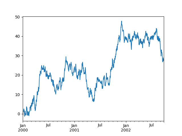
In [69]: ts = pd.Series(np.random.randn(1000),
   ....:                index=pd.date_range('1/1/2000', periods=1000))
   ....:

In [70]: ts = ts.cumsum()

In [71]: ts.plot()
Out[71]: <Axes: >
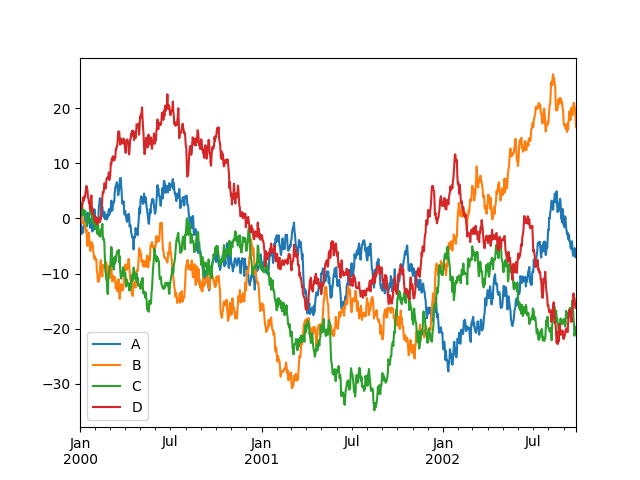
On a DataFrame, the plot() method is a convenience to plot all
of the columns with labels:
In [72]: df = pd.DataFrame(np.random.randn(1000, 4), index=ts.index,
   ....:                   columns=['A', 'B', 'C', 'D'])
   ....:

In [73]: df = df.cumsum()

In [74]: plt.figure()
Out[74]: <Figure size 640x480 with 0 Axes>

In [75]: df.plot()
Out[75]: <Axes: >

In [76]: plt.legend(loc='best')
Out[76]: <matplotlib.legend.Legend at 0x7fa9f6bfbd90>
Getting data in/out#
CSV#
Writing to a csv file.
In [77]: df.to_csv('foo.csv')
Out[77]:
Empty DataFrame
Columns: []
Index: []
Reading from a csv file.
In [78]: pd.read_csv('foo.csv')
Out[78]:
     Unnamed: 0         A          B          C          D
0    2000-01-01 -2.144314  -1.020917   0.775341   0.584840
1    2000-01-02 -1.376907   0.324642   1.403512   2.345983
2    2000-01-03 -0.890337   0.028875   2.799828   1.979749
3    2000-01-04 -2.825389   0.032440   2.444658   2.030794
4    2000-01-05 -2.054683   1.042795   2.352492   1.875531
..          ...       ...        ...        ...        ...
995  2002-09-22 -5.859770  20.952520 -19.344966 -14.540427
996  2002-09-23 -5.384162  20.266436 -21.277218 -14.517980
997  2002-09-24 -5.964959  19.935580 -20.495675 -15.598620
998  2002-09-25 -7.089211  18.178433 -20.508335 -16.279560
999  2002-09-26 -6.820622  16.567005 -19.695651 -16.248122

[1000 rows x 5 columns]